The filter option in Excel spreadsheets provides for an incredibly easy way to find and sort your data. But there are times when it can get a bit clunky, especially if you have a large range of different values, and you or your users are not comfortable with or familiar with all of the ways in which the data can be filtered. And what if your users want nothing to do with Excel but it's a requirement of their job to use it? This is where Visual Basic for Applications (VBA) comes in handy. With the simple click of a button (who can't do that?!), users can be presented with the data they need without having to dive (shallow or deeply) into any of Excel's robust features.
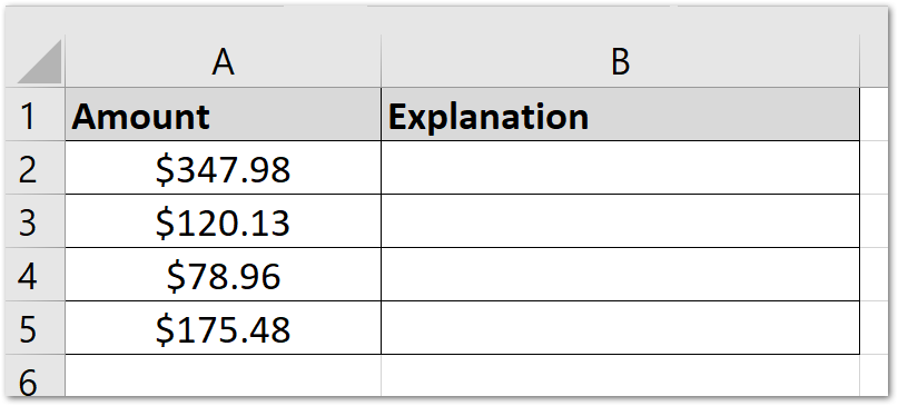
In this post, we're going to mimic the submission of invoice-type data in a corporate setting, but only after the salesperson has entered an explanation for any exceptions we identify. So let's say that you want a salesperson to only be able to submit his invoice report to the accounts receivable department only after he/she has added an explanation for each invoice less than $100.00. Perhaps there was a sale that week, a smaller order from the purchaser, or a discount was applied to the order. VBA allows for complex operations to be completed very simply with the use of Macros, functions, and the like.
Open up an Excel spreadsheet and get some data in columns A and B like so:
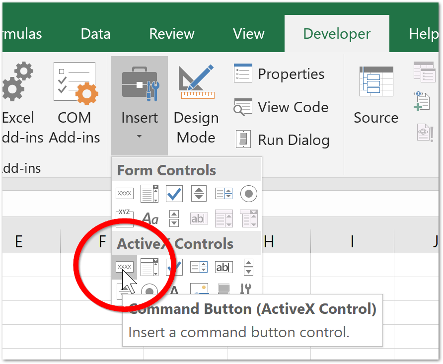
Then, go to the Developer tab and click the Insert option. Under ActiveX controls, select the icon to add a Command Button.
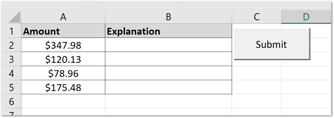
Draw the Command Button next to your data columns. Your spreadsheet will now change to Design Mode. Right click on the newly place command button, then hover over 'CommandButton Object' then click Edit to modify the label of the button. I changed mine to "Submit" because eventually this will be used to email the entire workbook.
Finally, right-click on the button and select 'View Code.' Copy and paste the below lines of code inbetween the 'Private Sub CommandButton1_Click()' and 'End Sub' lines.
Dim sht As Worksheet
Dim indicator As Boolean

Set sht = ThisWorkbook.Worksheets("Sheet1")
indicator = True
lastrow = sht.Cells(Rows.Count, "A").End(xlUp).Row

    ' Start at the second row, go until the last row that contains data
    For x = 2 To lastrow
        ' If the amount value is less than $100.00 AND there is no explanation
        ' Turn the exaplanation cell red as a visual indicator and change the indicator variable to false
        If sht.Cells(x, 1).Value < 100 And sht.Cells(x, 2).Value = "" Then
            sht.Cells(x, 2).Interior.ColorIndex = 22
            indicator = False
        End If
    Next x

    ' If any of the cells are < $100 and there is no comment, prompt the user to enter an explanation.
    If indicator = False Then
        MsgBox "One or more explanations is required before submission"
    Else
        ' Submit to ....
        MsgBox "SUCCESS! Submitted to A/R!"
    End If
Finally, we are ready to click that button. But first, make sure that your spreadsheet is not still in design mode by goign to the Developer tab and clicking Design Mode if it is currently selected.
The program cycles through all values in column A. If it finds a value less than $100.00 and no explanation in the cell next to it, it highlights the 'Explanation' cell, prompting the user to add an explanation, and changes the 'indicator' value to False. You could do this using a While (true) loop but the loop'll break after finding the first exception, only highlighting the first instance of a cell < $100.00. Instead, we loop through all of the data, highlight all of the exceptions, and evaluate the indicator variable at the end of the program. If there is an explanation for each value under $100, the indicator value remains True and the user is prompted with a 'Success' message box.

You can then extend the existing project to email the entire workbook using Ron de Bruin's Excel Automation Tips. A little bit of work on your part can significantly improve automation and efficiency in your environment, and allow your staff or volunteers to focus on what's important.